Process Monitoring with `TotalDepth.common.process`¶

TotalDepth.common.process can monitor the memory and CPU usage of a running process. It does this by creating a thread which, at regular intervals, reports process data to the log file in JSON. The basic use is like this:

from TotalDepth.common import process

with process.log_process(1.0):
    # Your code here

Then TotalDepth.common.process will write process data as a single line in the log file every 1.0 seconds. The JSON data is preceded by the following, recognisable, entry in the log file:

2019-10-31 14:10:06,051 - process.py - 86611 - (ProcMon   ) - INFO     - ProcessLoggingThread-JSON

The JSON data looks like this example (but on one line):

{
    "timestamp": "2019-10-31 14:10:06.051630",
    "memory_info":
        {
            "rss": 11939840,
            "vms": 4404228096,
            "pfaults": 531770,
            "pageins": 0
        },
    "cpu_times": {
        "user": 0.583945792,
        "system": 0.66087648,
        "children_user": 0.0,
        "children_system": 0.0
    },
    "elapsed_time": 12.42771601676941
}

Command Line Tools¶

Command line tools can add process capability with an argument parser created by TotalDepth.common.cmn_cmd_opts arg_parser():

process.add_process_logger_to_argument_parser(parser)

This makes the --log-process option available which takes a numeric value as a float in seconds (default zero which means no process logging) for the logging interval. Your code pattern is then:

args = parser.parse_args()
if args.log_process > 0.0:
    with process.log_process(args.log_process):
        # Do something

Plotting the Data¶

TotalDepth.common.process can be used from the command line to extract the data from the log file and plot it with Gnuplot.

Example¶

Here we will create eight large, randomly sized strings and simulate doing some work:

import random
import time

from TotalDepth.common import process

with process.log_process(0.1):
    for i in range(8):
        size = random.randint(128, 128 + 256) * 1024 ** 2
        s = ' ' * (size)
        # Simulate 0.5 to 1.5 seconds of work.
        time.sleep(0.5 + random.random())
        del s
        # Simulate 0.25 to 0.75 seconds of work.
        time.sleep(0.25 + random.random() / 2)

This will produce a log such as:

2019-10-31 14:09:53,726 - process.py - 86611 - (ProcMon   ) - INFO     - ProcessLoggingThread-JSON {"timestamp": "2019-10-31 14:09:53.726676", "memory_info": {"rss": 11898880, "vms": 4404228096, "pfaults": 3624, "pageins": 0}, "cpu_times": {"user": 0.07540488, "system": 0.020255324, "children_user": 0.0, "children_system": 0.0}, "elapsed_time": 0.10263395309448242}
2019-10-31 14:09:53,896 - process.py - 86611 - (ProcMon   ) - INFO     - ProcessLoggingThread-JSON {"timestamp": "2019-10-31 14:09:53.896083", "memory_info": {"rss": 162922496, "vms": 4555227136, "pfaults": 40495, "pageins": 0}, "cpu_times": {"user": 0.108017992, "system": 0.056484236, "children_user": 0.0, "children_system": 0.0}, "elapsed_time": 0.27210497856140137}
2019-10-31 14:09:53,997 - process.py - 86611 - (ProcMon   ) - INFO     - ProcessLoggingThread-JSON {"timestamp": "2019-10-31 14:09:53.996930", "memory_info": {"rss": 162930688, "vms": 4555227136, "pfaults": 40497, "pageins": 0}, "cpu_times": {"user": 0.10846144, "system": 0.05655662, "children_user": 0.0, "children_system": 0.0}, "elapsed_time": 0.373028039932251}
...
2019-10-31 14:10:06,051 - process.py - 86611 - (ProcMon   ) - INFO     - ProcessLoggingThread-JSON {"timestamp": "2019-10-31 14:10:06.051630", "memory_info": {"rss": 11939840, "vms": 4404228096, "pfaults": 531770, "pageins": 0}, "cpu_times": {"user": 0.583945792, "system": 0.66087648, "children_user": 0.0, "children_system": 0.0}, "elapsed_time": 12.42771601676941}

Then run TotalDepth.common.process CLI entry point with two arguments, the log file and a directory to write the Gnuplot data to.

$ python src/TotalDepth/common/process.py tmp/process_C.log tmp/gnuplot_process
2019-10-31 14:11:29,737 - gnuplot.py - 86631 - (MainThread) - INFO     - gnuplot stdout: None
2019-10-31 14:11:29,741 - gnuplot.py - 86631 - (MainThread) - INFO     - Writing gnuplot data "process_C.log" in path tmp/gnuplot_process
2019-10-31 14:11:29,782 - gnuplot.py - 86631 - (MainThread) - INFO     - gnuplot stdout: None

In the output directory there is the log data extracted as .dat file, the Gnuplot specification as .plt file, and the plot itself in SVG as process_C.log.svg:

$ ls -l tmp/gnuplot_process/
total 360
-rw-r--r--  1 xxxxxxxx  staff  13679 31 Oct 14:11 process_C.log.dat
-rw-r--r--  1 xxxxxxxx  staff   1067 31 Oct 14:11 process_C.log.plt
-rw-r--r--@ 1 xxxxxxxx  staff  30878 31 Oct 14:11 process_C.log.svg
-rw-r--r--  1 xxxxxxxx  staff  32100 31 Oct 14:11 test.svg

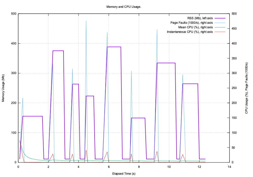
Here is process_C.log.svg:

Adding Events as Graph Labels¶

You can also inject events into TotalDepth.common.process as string messages and these will be reproduced on the plot as labels. So adding one line of code:

import random
import time

from TotalDepth.common import process

with process.log_process(0.1):
    for i in range(8):
        size = random.randint(128, 128 + 256) * 1024 ** 2
        process.add_message_to_queue(f'String of {size:,d} bytes')
        s = ' ' * (size)
        # Simulate 0.5 to 1.5 seconds of work.
        time.sleep(0.5 + random.random())
        del s
        # Simulate 0.25 to 0.75 seconds of work.
        time.sleep(0.25 + random.random() / 2)

Adds that label into the JSON on the next write:

{
    "label": 'String of xxx bytes'
    # ...
}

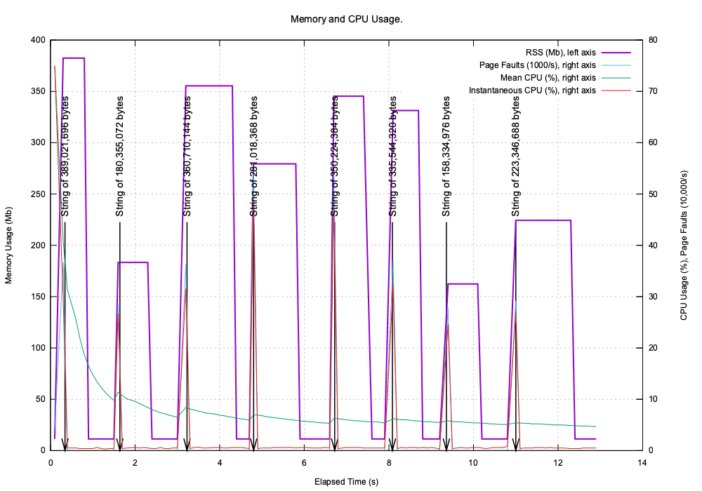
When plotted these labels appear on the plot:

A Real World Example¶

Here is an example of running TotalDepth.RP66V1.ScanHTML on four files of sizes 75, 80, 8 and 500 MB. TotalDepth.RP66V1.ScanHTML essentially does two things:

Creates an index of the RP66V1 file.
Then iterates across that index writing HTML, this includes reading a (potentially) large number of frames depending on the file.

The start points of these operations are labeled on the graph.

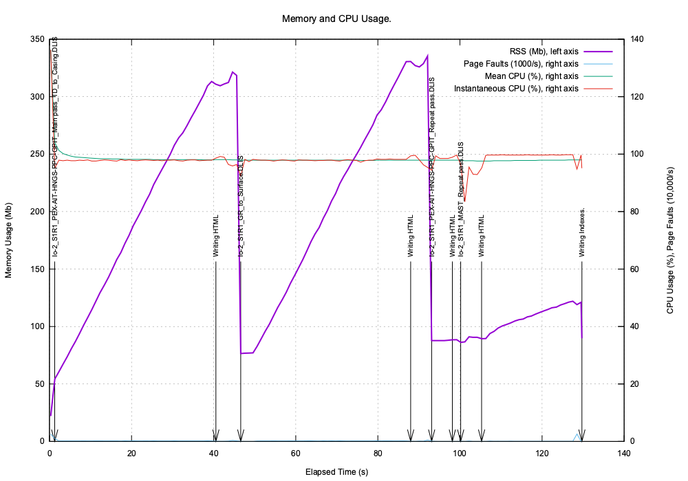
The graphs clearly shows that for the last file reading the index is very quick but writing the HTML is comparatively slow. This is because that is an unusual file that deserves further investigation.

Process Monitoring with TotalDepth.common.process¶