Plotting Wireline Data
Aside from the LogPass (the data structure that holds the frame data) the plot layout needs to be specified. There are two ways that TotalDepth does this:
- A plot specification that is integral to the file. For example; LIS files may well have FILM and PRES tables within them that configure the plot as the recording engineer (or software) intended. In this case TotalDepth can make those plots directly.
- A plot specification that is specified externally to the file. TotalDepth supports one such way; using LgFormat XML files and these are described below.
Wireline Files With Integral Plot Data
This applies to LIS (and possibly RP66 files). The LAS file specification does not describe any plot specification at all.
LIS Plot Specification
There are a number of table-like Logical Records (type 34) within a Log Pass that can specify the plot layout. As a minimum TotalDepth.LIS needs a FILM and a PRES record.
FILM Record
A dump of a FILM Logical Record might look like this:
Table record (type 34) type: FILM

MNEM  GCOD  GDEC  DEST  DSCA
-----------------------------

1     EEE   ----  PF2   D200
2     E4E   -4--  PF1   DM
The columns are:
| Column | Description |
|---|---|
MNEM |
The (logical) name of the output, TotalDepth uses this as part of the plot file name. |
GCOD |
The coding of the tracks. E4E means three tracks which have linear, log (4 decades), linear.
With three tracks the X axis track (depth for example) appears between the first and second tracks. |
GDEC |
The number of logarithmic decades for each track, - for linear. |
DEST |
The physical destination (in the logging unit) of the plot. Ignored. |
DSCA |
The depth scale, encoded. For example D200 means 1:200. |
PRES Record
A dump of a PRES Logical Record might look like this:
 Table record (type 34) type: PRES

MNEM  OUTP  STAT  TRAC  CODI  DEST  MODE      FILT          LEDG          REDG
-----------------------------------------------------------------------------------

SP    SP    ALLO  T1    LLIN  1     SHIF      0.500000      -80.0000       20.0000
CALI  CALI  ALLO  T1    LDAS  1     SHIF      0.500000       5.00000       15.0000
MINV  MINV  DISA  T1    LLIN  1     SHIF      0.500000       30.0000       0.00000
MNOR  MNOR  DISA  T1    LDAS  1     SHIF      0.500000       30.0000       0.00000
LLD   LLD   ALLO  T23   LDAS  1     GRAD      0.500000      0.200000       2000.00
LLDB  LLD   ALLO  T2    HDAS  1     GRAD      0.500000       2000.00       200000.
LLG   LLG   DISA  T23   LDAS  1     GRAD      0.500000      0.200000       2000.00
LLGB  LLG   DISA  T2    HDAS  1     GRAD      0.500000       2000.00       200000.
LLS   LLS   ALLO  T23   LSPO  1     GRAD      0.500000      0.200000       2000.00
LLSB  LLS   ALLO  T2    HSPO  1     GRAD      0.500000       2000.00       200000.
MSFL  MSFL  ALLO  T23   LLIN  1     GRAD      0.500000      0.200000       2000.00
11    DUMM  DISA  T1    LLIN  NEIT  NB        0.500000       0.00000       1.00000
12    DUMM  DISA  T1    LLIN  NEIT  NB        0.500000       0.00000       1.00000
...
| Column | Description |
|---|---|
MNEM |
The (logical) name of the output curve. Note multiple curves might come from one OUTP. |
OUTP |
The source of the curve. |
STAT |
Status, is this curve to be plotted. |
TRAC |
Which track the curve should be plotted on. |
CODE |
The line coding, dot, dash etc. |
DEST |
The logical film that this curve is sent to. Can be BOTH and so on. |
MODE |
What to do when the curve goes off scale (wrap round the track for example). |
FILT |
Filtering. Unused. |
LEDG |
Value of the left edge of the plot. |
REDG |
Value of the right edge of the plot. |
Records Needed for a LIS Plot
As a minimum TotalDepth needs a FILM and PRES plot, using these TotalDepth can produce a plot identical to that when the data was recorded.
In future releases TotalDepth might also support these Logical Records for plotting:
AREA: Describes shading between curves on a plot.PIP: Describes integration marks on the plot such as integrated transit time, integrated hole volume etc.VDL: Describes presentation of waveform amplitude data.
Wireline Files With External Plot Data
This can apply to any wireline file and it means using an external configuration file to decide the plot layout. For example; LAS files do not have any plot specification (the LAS standard precludes this). The presentation of the plot is made with an external plot specification.
These external plot specifications are numerous and varied. TotalDepth currently supports one such specification: the XML LgFormat or LgSchema files.
LgFormat XML Files
These appear to originate from some of Schlumberger’s “free” software.
Here is an example LgFormat XML file for plotting HDT logs .TotalDepth supplies an number of examples of these.
There are a number of problems [1] with the LgFormat which is why TotalDepth only supports a subset of it while we look for something better.
Internal Plot Algorithms
This describes some algorithms used by the Plot module. This is for information only as these algorithms are internal and the user has little or no control over them.
Plotting the Legends (Scales)
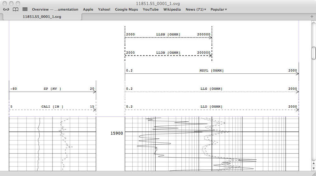
These at each end of the plot per curve and may span a number of tracks or be limited to half a track. Here is an example which has seven curves:
TODO: Finish this
There are two important methods that implement this algorithm: Plot.Plot._retCurvePlotScaleOrder() and Plot.Plot._plotScale()
Interpolating Backups
Industry standard wireline plots have the notion of curve backups where if the the trace for a particular curve goes off scale on one side of the track it might well reappear from the alternate side.
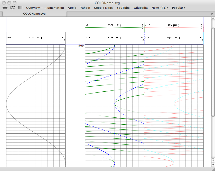
Here is a simulated example generated by TestPlot.py where a single curve (a sin curve with an amplitude of +/- 40) is plotted in full on track one. The same curve is plotted fully backed up:
- In green on track two with a scale of +/- 5
- In blue on track two with a scale of +/- 20
- In red on track three with a scale of +/- 2.5
- In aqua on track three with a scale of +/- 10
The algorithm that does this is probably best illustrated by example. The diagram below shows a curve (in the white track on the left) that goes from from point A goes off-scale to the right to point B in ‘real’ space. The line A-B is subdivided by track widths and these crossing lines are plotted by interpolation in the track space making the line space A-B’ (so-called ‘FlyBack’ lines are omitted in the diagram). If the Backup Mode is wrap then both red and green lines in the track are plotted. In this case if the Backup Mode is 1 then only the red lines are plotted in the track i.e. only one backup allowed.
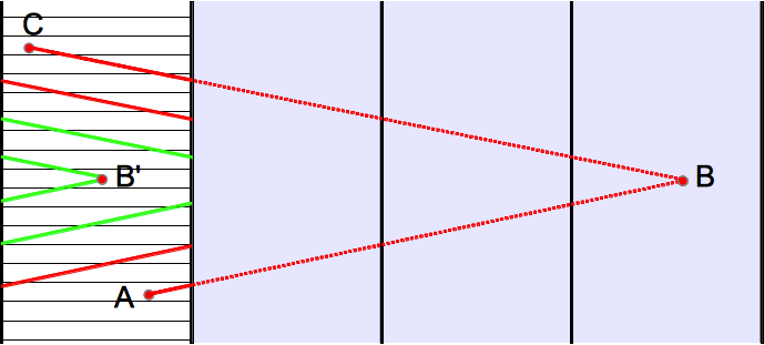
On the return B-C a similar process happens in reverse.
Backup Specification
A backup specification is expected for any plot per-curve. Internally a backup specification is a pair of integers. If the virtual track position is less than the value (if left) or greater than the value (if right) then it is off scale. Zero is a special case in that all virtual track positions are on scale.
Various values have been predefined and there are existing mappings from LIS data and LgFormat XML files. The following table describes all of this.
| Spec. | Symbol | Description | LIS Mapping | LgFormat Mapping |
|---|---|---|---|---|
| (1, -1) | BACKUP_NONE | No backup | ‘NB ‘, ‘GRAD’ | |
| (0, 0) | BACKUP_ALL | Every backup i.e. ‘wrap’ Note: Plot.py has a way of limiting ludicrous backup lines to a sensible number; say 4 | ‘WRAP’ | ‘LG_WRAPPED’ ‘LG_X10’ |
| (-1, 1) | BACKUP_ONCE | Single backup to left or right | ‘SHIF’ | ‘1’ |
| (-2, 2) | BACKUP_TWICE | Two backups to left or right | ‘2’ | |
| (0, -1) | BACKUP_LEFT | Single backup to left only | ‘LG_LEFT_WRAPPED’ | |
| (1, 0) | BACKUP_RIGHT | Single backup to right only | ‘LG_RIGHT_WRAPPED’ |
Note that it is also common to have one curve with no backup and a second curve driven from the same output with a different scale acting as a backup. This has the advantage that a different coding and colour can be assigned to it. See Plotting the Legends (Scales) above for an example with a Laterlog plot.
Algorithm
The backup algorithm works as follows:
- For every point plotted an integer wrap value is calculated.
- If the wrap value is different from the previous wrap value then some interpolation is required and the
Plot._interpolateBackup()method is called (below). - Otherwise the point is plotted.
_interpolateBackup
The Plot._interpolateBackup() method manages all the different cases where a backup is needed given the backup configuration. It relies on Plot._retInterpolateWrapPoints() to generate a list of interpolated lines, including crossing lines, between one point and another.
_filterCrossLineList
A further refinement to the algorithm is limiting the number of crossing lines. Consider the SP curve represented by this data taken from a real example:
Depth (ft) SP (mV)
10245.0    332.724
10245.5    13716948.000
10246.0    41150204.000
10246.5    68583456.000
10247.0    96016712.000
10247.5    334.176
Clearly some episode happened between 10245.0 and 10245.5 feet that caused a jump of 13716615.276 mV. This could have been an recording disturbance (unlikely as where would you find 96kV at 10247 feet?) or an editing error. In any case on a scale of -20 to 80 mV means 137,166 (mostly spurious) wrap lines crossing the track. This can turn a 1.6Mb file into a 91Mb file! To stop this a arbitrary limit is made to the number of crossing lines (e.g. 4) between each Xaxis interval. This limit filters the crossing line list to an evenly distributed list of 4 (or thereabouts).
This is also applicable to RFT plots where it is common to plot the pressure modulo 10 psi in RHT3.
The method that does this is The Plot._filterCrossLineList() method
Footnotes
| [1] | For example the LgCurve element content of <LeftLimit> and <RightLimit> is numeric, without units. This robs a compliant implementation of the opportunity of converting frame data, say in "V/V " to plot data say "PU " which might be far more appropriate. Truth in advertising prompts me to say that LIS PRES tables have the same flaw but they have a reasonable excuse that they are per file specification rather than a global specification. |